Bloom filter
| Part of a series on |
| Probabilistic data structures |
|---|
| Bloom filter · Skip list |
| Random trees |
| Rapidly-exploring random tree |
| Related |
| Randomized algorithm |
| Computer science Portal |
A Bloom filter, conceived by Burton Howard Bloom in 1970,[1] is a space-efficient probabilistic data structure that is used to test whether an element is a member of a set. False positives are possible, but false negatives are not; i.e. a query returns either "inside set (may be wrong)" or "definitely not in set". Elements can be added to the set, but not removed (though this can be addressed with a counting filter). The more elements that are added to the set, the larger the probability of false positives.
Contents |
Algorithm description
An empty Bloom filter is a bit array of m bits, all set to 0. There must also be k different hash functions defined, each of which maps or hashes some set element to one of the m array positions with a uniform random distribution.
To add an element, feed it to each of the k hash functions to get k array positions. Set the bits at all these positions to 1.
To query for an element (test whether it is in the set), feed it to each of the k hash functions to get k array positions. If any of the bits at these positions are 0, the element is not in the set – if it were, then all the bits would have been set to 1 when it was inserted. If all are 1, then either the element is in the set, or the bits have been set to 1 during the insertion of other elements.
The requirement of designing k different independent hash functions can be prohibitive for large k. For a good hash function with a wide output, there should be little if any correlation between different bit-fields of such a hash, so this type of hash can be used to generate multiple "different" hash functions by slicing its output into multiple bit fields. Alternatively, one can pass k different initial values (such as 0, 1, ..., k − 1) to a hash function that takes an initial value; or add (or append) these values to the key. For larger m and/or k, independence among the hash functions can be relaxed with negligible increase in false positive rate (Dillinger & Manolios (2004a), Kirsch & Mitzenmacher (2006)). Specifically, Dillinger & Manolios (2004b) show the effectiveness of deriving the k indices using enhanced double hashing or triple hashing, variants of double hashing that are effectively simple random number generators seeded with the two or three hash values.
Removing an element from this simple Bloom filter is impossible because false negatives are not permitted. An element maps to k bits, and although setting any one of those k bits to zero suffices to remove the element, it also results in removing any other elements that happen to map onto that bit. Since there is no way of determining whether any other elements have been added that affect the bits for an element to be removed, clearing any of the bits would introduce the possibility for false negatives.
One-time removal of an element from a Bloom filter can be simulated by having a second Bloom filter that contains items that have been removed. However, false positives in the second filter become false negatives in the composite filter, which are not permitted. In this approach re-adding a previously removed item is not possible, as one would have to remove it from the "removed" filter.
However, it is often the case that all the keys are available but are expensive to enumerate (for example, requiring many disk reads). When the false positive rate gets too high, the filter can be regenerated; this should be a relatively rare event.
Space and time advantages
While risking false positives, Bloom filters have a strong space advantage over other data structures for representing sets, such as self-balancing binary search trees, tries, hash tables, or simple arrays or linked lists of the entries. Most of these require storing at least the data items themselves, which can require anywhere from a small number of bits, for small integers, to an arbitrary number of bits, such as for strings (tries are an exception, since they can share storage between elements with equal prefixes). Linked structures incur an additional linear space overhead for pointers. A Bloom filter with 1% error and an optimal value of k, in contrast, requires only about 9.6 bits per element — regardless of the size of the elements. This advantage comes partly from its compactness, inherited from arrays, and partly from its probabilistic nature. If a 1% false-positive rate seems too high, adding about 4.8 bits per element decreases it by ten times.
However, if the number of potential values is small and many of them can be in the set, the Bloom filter is easily surpassed by the deterministic bit array, which requires only one bit for each potential element. Note also that hash tables gain a space and time advantage if they begin ignoring collisions and store only whether each bucket contains an entry; in this case, they have effectively become Bloom filters with k = 1.
Bloom filters also have the unusual property that the time needed either to add items or to check whether an item is in the set is a fixed constant, O(k), completely independent of the number of items already in the set. No other constant-space set data structure has this property, but the average access time of sparse hash tables can make them faster in practice than some Bloom filters. In a hardware implementation, however, the Bloom filter shines because its k lookups are independent and can be parallelized.
To understand its space efficiency, it is instructive to compare the general Bloom filter with its special case when k = 1. If k = 1, then in order to keep the false positive rate sufficiently low, a small fraction of bits should be set, which means the array must be very large and contain long runs of zeros. The information content of the array relative to its size is low. The generalized Bloom filter (k greater than 1) allows many more bits to be set while still maintaining a low false positive rate; if the parameters (k and m) are chosen well, about half of the bits will be set, and these will be apparently random, minimizing redundancy and maximizing information content.
Probability of false positives
Assume that a hash function selects each array position with equal probability. If m is the number of bits in the array, the probability that a certain bit is not set to one by a certain hash function during the insertion of an element is then

The probability that it is not set by any of the hash functions is
If we have inserted n elements, the probability that a certain bit is still 0 is
the probability that it is 1 is therefore
Now test membership of an element that is not in the set. Each of the k array positions computed by the hash functions is 1 with a probability as above. The probability of all of them being 1, which would cause the algorithm to erroneously claim that the element is in the set, is often given as
![\left(1-\left[1-\frac{1}{m}\right]^{kn}\right)^k \approx \left( 1-e^{-kn/m} \right)^k.](/2012-wikipedia_en_all_nopic_01_2012/I/2180ac79da81e5b3721963b4d80cf5a6.png)
This is not strictly correct as it assumes independence for the probabilities of each bit being set. However, assuming it is a close approximation we have that the probability of false positives decreases as m (the number of bits in the array) increases, and increases as n (the number of inserted elements) increases. For a given m and n, the value of k (the number of hash functions) that minimizes the probability is
which gives the false positive probability of

The required number of bits m, given n (the number of inserted elements) and a desired false positive probability p (and assuming the optimal value of k is used) can be computed by substituting the optimal value of k in the probability expression above:
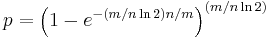
which can be simplified to:
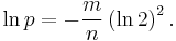
This results in:
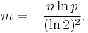
This means that in order to maintain a fixed false positive probability, the length of a Bloom filter must grow linearly with the number of elements being filtered. While the above formula is asymptotic (i.e. applicable as m, n → ∞), the agreement with finite values of m,n is also quite good; the false positive probability for a finite bloom filter with m bits, n elements, and k hash functions is at most
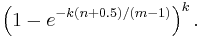
So we can use the asymptotic formula if we pay a penalty for at most half an extra element and at most one fewer bit Goel & Gupta (2010).
Interesting properties
- Unlike sets based on hash tables, any Bloom filter can represent the entire universe of elements. In this case, all bits are 1. Another consequence of this property is that add never fails due to the data structure "filling up." However, the false positive rate increases steadily as elements are added until all bits in the filter are set to 1, so a negative value is never returned. At this point, the Bloom filter completely ceases to differentiate between differing inputs, and is functionally useless.
- Union and intersection of Bloom filters with the same size and set of hash functions can be implemented with bitwise OR and AND operations, respectively. The union operation on Bloom filters is lossless in the sense that the resulting Bloom filter is the same as the Bloom filter created from scratch using the union of the two sets. The intersect operation satisfies a weaker property: the false positive probability in the resulting Bloom filter is at most the false-positive probability in one of the constituent Bloom filters, but may be larger than the false positive probability in the Bloom filter created from scratch using the intersection of the two sets.
Examples
Google BigTable uses Bloom filters to reduce the disk lookups for non-existent rows or columns. Avoiding costly disk lookups considerably increases the performance of a database query operation.[2]
The Squid Web Proxy Cache uses Bloom filters for cache digests.[3]
The Venti archival storage system uses Bloom filters to detect previously-stored data.[4]
The SPIN model checker uses Bloom filters to track the reachable state space for large verification problems.[5]
The Google Chrome web browser uses Bloom filters to speed up its Safe Browsing service.[6]
Alternatives
Classic Bloom filters use  bits of space per inserted key, where
  is the false positive rate of the Bloom filter. However, the space that is strictly necessary for any data structure playing the same role as a Bloom filter is only
  per key (Pagh, Pagh & Rao 2005). Hence Bloom filters use 44% more space than a hypothetical equivalent optimal data structure. The number of hash functions used to achieve a given false positive rate is proportional to
  which is not optimal as it has been proved that an optimal data structure would need only a constant number of hash functions independent of the false positive rate.
Stern & Dill (1996) describe a probabilistic structure based on hash tables, hash compaction, which Dillinger & Manolios (2004b) identify as significantly more accurate than a Bloom filter when each is configured optimally. Dillinger and Manolios, however, point out that the reasonable accuracy of any given Bloom filter over a wide range of numbers of additions makes it attractive for probabilistic enumeration of state spaces of unknown size. Hash compaction is, therefore, attractive when the number of additions can be predicted accurately; however, despite being very fast in software, hash compaction is poorly-suited for hardware because of worst-case linear access time.
Putze, Sanders & Singler (2007) have studied some variants of Bloom filters that are either faster or use less space than classic Bloom filters. The basic idea of the fast variant is to locate the k hash values associated with each key into one or two blocks having the same size as processor's memory cache blocks (usually 64 bytes). This will presumably improve performance by reducing the number of potential memory cache misses. The proposed variants have however the drawback of using about 32% more space than classic Bloom filters.
The space efficient variant relies on using a single hash function that generates for each key a value in the range ![\left[0,n/\varepsilon\right]](/2012-wikipedia_en_all_nopic_01_2012/I/8719561052ee96a6f1c88ae38a05dbe2.png) where is the requested false positive rate. The sequence of values is then sorted and compressed using Golomb coding (or some other compression technique) to occupy a space close to
where is the requested false positive rate. The sequence of values is then sorted and compressed using Golomb coding (or some other compression technique) to occupy a space close to  bits. To query the Bloom filter for a given key, it will suffice to check if its corresponding value is stored in the Bloom filter. Decompressing the whole Bloom filter for each query would make this variant totally unusable. To overcome this problem the sequence of values is divided into small blocks of equal size that are compressed separately. At query time only half a block will need to be decompressed on average. Because of decompression overhead, this variant may be slower than classic Bloom filters but this may be compensated by the fact that a single hash function need to be computed.
Another alternative to classic Bloom filter is the one based on space efficient variants of cuckoo hashing. In this case once the hash table is constructed, the keys stored in the hash table are replaced with short signatures of the keys. Those signatures are strings of bits computed using a hash function applied on the keys.
Extensions and applications
Counting filters
Counting filters provide a way to implement a delete operation on a Bloom filter without recreating the filter afresh. In a counting filter the array positions (buckets) are extended from being a single bit, to an n-bit counter. In fact, regular Bloom filters can be considered as counting filters with a bucket size of one bit. Counting filters were introduced by Fan et al. (1998).
The insert operation is extended to increment the value of the buckets and the lookup operation checks that each of the required buckets is non-zero. The delete operation, obviously, then consists of decrementing the value of each of the respective buckets.
Arithmetic overflow of the buckets is a problem and the buckets should be sufficiently large to make this case rare. If it does occur then the increment and decrement operations must leave the bucket set to the maximum possible value in order to retain the properties of a Bloom filter.
The size of counters is usually 3 or 4 bits. Hence counting Bloom filters use 3 to 4 times more space than static Bloom filters. In theory, an optimal data structure equivalent to a counting Bloom filter should not use more space than a static Bloom filter.
Another issue with counting filters is limited scalability. Because the counting Bloom filter table cannot be expanded, the maximal number of keys to be stored simultaneously in the filter must be known in advance. Once the designed capacity of the table is exceeded the false positive rate will grow rapidly as more keys are inserted.
Bonomi et al. (2006) introduced a data structure based on d-left hashing that is functionally equivalent but uses approximately half as much space as counting Bloom filters. The scalability issue does not occur in this data structure. Once the designed capacity is exceeded, the keys could be reinserted in a new hash table of double size.
The space efficient variant by Putze, Sanders & Singler (2007) could also be used to implement counting filters by supporting insertions and deletions.
Data synchronization
Bloom filters can be used for approximate data synchronization as in Byers et al. (2004). Counting Bloom filters can be used to approximate the number of differences between two sets and this approach is described in Agarwal & Trachtenberg (2006).
Bloomier filters
Chazelle et al. (2004) designed a generalization of Bloom filters that could associate a value with each element that had been inserted, implementing an associative array. Like Bloom filters, these structures achieve a small space overhead by accepting a small probability of false positives. In the case of "Bloomier filters", a false positive is defined as returning a result when the key is not in the map. The map will never return the wrong value for a key that is in the map.
The simplest Bloomier filter is near-optimal and fairly simple to describe. Suppose initially that the only possible values are 0 and 1. We create a pair of Bloom filters A0 and B0 which contain, respectively, all keys mapping to 0 and all keys mapping to 1. Then, to determine which value a given key maps to, we look it up in both filters. If it is in neither, then the key is not in the map. If the key is in A0 but not B0, then it does not map to 1, and has a high probability of mapping to 0. Conversely, if the key is in B0 but not A0, then it does not map to 0 and has a high probability of mapping to 1.
A problem arises, however, when both filters claim to contain the key. We never insert a key into both, so one or both of the filters is lying (producing a false positive), but we don't know which. To determine this, we have another, smaller pair of filters A1 and B1. A1 contains keys that map to 0 and which are false positives in B0; B1 contains keys that map to 1 and which are false positives in A0. But whenever A0 and B0 both produce positives, at most one of these cases must occur, and so we simply have to determine which if any of the two filters A1 and B1 contains the key, another instance of our original problem.
It may so happen again that both filters produce a positive; we apply the same idea recursively to solve this problem. Because each pair of filters only contains keys that are in the map and produced false positives on all previous filter pairs, the number of keys is extremely likely to quickly drop to a very small quantity that can be easily stored in an ordinary deterministic map, such as a pair of small arrays with linear search. Moreover, the average total search time is a constant, because almost all queries will be resolved by the first pair, almost all remaining queries by the second pair, and so on. The total space required is independent of n, and is almost entirely occupied by the first filter pair.
Now that we have the structure and a search algorithm, we also need to know how to insert new key/value pairs. The program must not attempt to insert the same key with both values. If the value is 0, insert the key into A0 and then test if the key is in B0. If so, this is a false positive for B0, and the key must also be inserted into A1 recursively in the same manner. If we reach the last level, we simply insert it. When the value is 1, the operation is similar but with A and B reversed.
Now that we can map a key to the value 0 or 1, how does this help us map to general values? This is simple. We create a single such Bloomier filter for each bit of the result. If the values are large, we can instead map keys to hash values that can be used to retrieve the actual values. The space required for a Bloomier filter with n-bit values is typically slightly more than the space for 2n Bloom filters.
A very simple way to implement Bloomier filters is by means of minimal perfect hashing. A minimal perfect hash function h is first generated for the set of n keys. Then an array is filled with n pairs (signature,value) associated with each key at the positions given by function h when applied on each key. The signature of a key is a string of r bits computed by applying a hash function g of range  on the key. The value of r is chosen such that
  , where is the requested false positive rate. To query for a given key, hash function h is first applied on the key. This will give a position into the array from which we retrieve a pair (signature,value). Then we compute the signature of the key using function g. If the computed signature is the same as retrieved signature we return the retrieved value. The probability of false positive is
  .
.
Another alternative to implement static bloomier and bloom filters based on matrix solving has been simultaneously proposed in Porat (2008) , Dietzfelbinger & Pagh (2008) and Charles & Chellapilla (2008). The space usage of this method is optimal as it needs only  bits per key for a bloom filter. However time to generate the bloom or bloomier filter can be very high. The generation time can be reduced to a reasonable value at the price of a small increase in space usage.
Dynamic Bloomier filters have been studied by Mortensen, Pagh & Pătraşcu (2005). They proved that any dynamic Bloomier filter needs at least around  bits per key where l is the length of the key. A simple dynamic version of Bloomier filters can be implemented using two dynamic data structures. Let the two data structures be noted S1 and S2. S1 will store keys with their associated data while S2 will only store signatures of keys with their associated data. Those signatures are simply hash values of keys in the range
 ![[0,n/\varepsilon]](/2012-wikipedia_en_all_nopic_01_2012/I/d1a01f1a6ceceb0621291cf33889d743.png) where n is the maximal number of keys to be stored in the Bloomier filter and is the requested false positive rate. To insert a key in the Bloomier filter, its hash value is first computed. Then the algorithm checks if a key with the same hash value already exists in S2. If this is not the case, the hash value is inserted in S2 along with data associated with the key. If the same hash value already exists in S2 then the key is inserted into S1 along with its associated data. The deletion is symmetric: if the key already exists in S1 it will be deleted from there, otherwise the hash value associated with the key is deleted from S2. An issue with this algorithm is on how to store efficiently S1 and S2. For S1 any hash algorithm can be used. To store S2 golomb coding could be applied to compress signatures to use a space close to
where n is the maximal number of keys to be stored in the Bloomier filter and is the requested false positive rate. To insert a key in the Bloomier filter, its hash value is first computed. Then the algorithm checks if a key with the same hash value already exists in S2. If this is not the case, the hash value is inserted in S2 along with data associated with the key. If the same hash value already exists in S2 then the key is inserted into S1 along with its associated data. The deletion is symmetric: if the key already exists in S1 it will be deleted from there, otherwise the hash value associated with the key is deleted from S2. An issue with this algorithm is on how to store efficiently S1 and S2. For S1 any hash algorithm can be used. To store S2 golomb coding could be applied to compress signatures to use a space close to  per key.
Compact approximators
Boldi & Vigna (2005) proposed a lattice-based generalization of Bloom filters. A compact approximator associates to each key an element of a lattice (the standard Bloom filters being the case of the Boolean two-element lattice). Instead of a bit array, they have an array of lattice elements. When adding a new association between a key and an element of the lattice, they maximize the current content of the k array locations associated to the key with the lattice element. When reading the value associated to a key, they minimize the values found in the k locations associated to the key. The resulting value approximates from above the original value.
Stable Bloom filters
Deng & Rafiei (2006) proposed Stable Bloom filters as a variant of Bloom filters for streaming data. The idea is that since there is no way to store the entire history of a stream (which can be infinite), Stable Bloom filters continuously evict stale information to make room for more recent elements. Since stale information is evicted, the Stable Bloom filter introduces false negatives, which do not appear in traditional bloom filters. The authors show that a tight upper bound of false positive rates is guaranteed, and the method is superior to standard bloom filters in terms of false positive rates and time efficiency when a small space and an acceptable false positive rate are given.
Scalable Bloom filters
Almeida et al. (2007) proposed a variant of Bloom filters that can adapt dynamically to the number of elements stored, while assuring a minimum false positive probability. The technique is based on sequences of standard bloom filters with increasing capacity and tighter false positive probabilities, so as to ensure that a maximum false positive probability can be set beforehand, regardless of the number of elements to be inserted.
Attenuated Bloom filters
An attenuated bloom filter of depth D can be viewed as an array of D normal bloom filters. In the context of service discovery in a network, each node stores regular and attenuated bloom filters locally. The regular or local bloom filter indicates which services are offered by the node itself. The attenuated filter of level i indicates which services can be found on nodes that are i-hops away from the current node. The i-th value is constructed by taking a union of local bloom filters for nodes i-hops away from the node. [7]
Lets take a small network shown on the graph below as an example. Say we are searching for a service A whose id hashes to bits 0,1, and 3 (pattern 11010). Let n1 node to be the starting point. First, we check whether service A is offered by n1 by checking its local filter. Since the patterns don't match, we check the attenuated bloom filter in order to determine which node should be the next hop. We see that n2 doesn't offer service A but lies on the path to nodes that do. Hence, we move to n2 and repeat the same procedure. We quickly find that n3 offers the service, and hence the destination is located. [8]
By using attenuated Bloom filters consisting of multiple layers, services at more than one hop distance can be discovered while avoiding saturation of the Bloom filter by attenuating (shifting out) bits set by sources further away. [9]
Notes
- ^ Donald Knuth. "The Art of Computer Programming, Errata for Volume 3 (2nd ed.)". http://www-cs-faculty.stanford.edu/~knuth/err3.textxt.
- ^ (Chang et al. 2006).
- ^ Wessels, Duane (January 2004), "10.7 Cache Digests", Squid: The Definitive Guide (1st ed.), O'Reilly Media, p. 172, ISBN 0596001622, "Cache Digests are based on a technique first published by Pei Cao, called Summary Cache. The fundamental idea is to use a Bloom filter to represent the cache contents."
- ^ http://plan9.bell-labs.com/magic/man2html/8/venti
- ^ http://spinroot.com/
- ^ http://src.chromium.org/viewvc/chrome/trunk/src/chrome/browser/safe_browsing/bloom_filter.h?view=markup
- ^ Koucheryavy et al. (Braun)
- ^ Kubiatowicz et al. (Eaton)
- ^ Koucheryavy et al. (Braun)
References
- Koucheryavy, Y.; Giambene, G.; Staehle, D.; Barcelo-Arroyo, F.; Braun, T.; Siris, V. (2009), "Traffic and QoS Management in Wireless Multimedia Networks", COST 290 Final Report (USA): 111, doi:XVI, 312
- Kubiatowicz, J.; Bindel, D.; Czerwinski, Y.; Geels, S.; Eaton, D.; Gummadi, R.; Rhea, S.; Weatherspoon, H. et al. (2000), "Oceanstore: An architecture for global-scale persistent storage", ACM SIGPLAN NOTICES (USA): 190-201, doi:2000, VOL 35; PART 11, http://ftp.csd.uwo.ca/courses/CS9843b/papers/OceanStore.pdf
- Agarwal, Sachin; Trachtenberg, Ari (2006), "Approximating the number of differences between remote sets", IEEE Information Theory Workshop (Punta del Este, Uruguay): 217, doi:10.1109/ITW.2006.1633815, http://www.deutsche-telekom-laboratories.de/~agarwals/publications/itw2006.pdf
- Ahmadi, Mahmood; Wong, Stephan (2007), "A Cache Architecture for Counting Bloom Filters", 15th international Conference on Netwroks (ICON-2007), pp. 218, doi:10.1109/ICON.2007.4444089, http://www.ieeexplore.ieee.org/xpls/abs_all.jsp?isnumber=4444031&arnumber=4444089&count=113&index=57
- Almeida, Paulo; Baquero, Carlos; Preguica, Nuno; Hutchison, David (2007), "Scalable Bloom Filters", Information Processing Letters 101 (6): 255–261, doi:10.1016/j.ipl.2006.10.007, http://gsd.di.uminho.pt/members/cbm/ps/dbloom.pdf
- Byers, John W.; Considine, Jeffrey; Mitzenmacher, Michael; Rost, Stanislav (2004), "Informed content delivery across adaptive overlay networks", IEEE/ACM Transactions on Networking 12 (5): 767, doi:10.1109/TNET.2004.836103
- Bloom, Burton H. (1970), "Space/time trade-offs in hash coding with allowable errors", Communications of the ACM 13 (7): 422–426, doi:10.1145/362686.362692
- Boldi, Paolo; Vigna, Sebastiano (2005), "Mutable strings in Java: design, implementation and lightweight text-search algorithms", Science of Computer Programming 54 (1): 3–23, doi:10.1016/j.scico.2004.05.003
- Bonomi, Flavio; Mitzenmacher, Michael; Panigrahy, Rina; Singh, Sushil; Varghese, George (2006), "An Improved Construction for Counting Bloom Filters", Algorithms – ESA 2006, 14th Annual European Symposium, 4168, pp. 684–695, doi:10.1007/11841036_61, http://theory.stanford.edu/~rinap/papers/esa2006b.pdf
- Broder, Andrei; Mitzenmacher, Michael (2005), "Network Applications of Bloom Filters: A Survey", Internet Mathematics 1 (4): 485–509, http://www.eecs.harvard.edu/~michaelm/postscripts/im2005b.pdf
- Chang, Fay; Dean, Jeffrey; Ghemawat, Sanjay; Hsieh, Wilson; Wallach, Deborah; Burrows, Mike; Chandra, Tushar; Fikes, Andrew et al. (2006), "Bigtable: A Distributed Storage System for Structured Data", Seventh Symposium on Operating System Design and Implementation, http://research.google.com/archive/bigtable.html
- Charles, Denis; Chellapilla, Kumar (2008), "Bloomier Filters: A second look", The Computing Research Repository (CoRR), arXiv:0807.0928
- Chazelle, Bernard; Kilian, Joe; Rubinfeld, Ronitt; Tal, Ayellet (2004), "The Bloomier filter: an efficient data structure for static support lookup tables", Proceedings of the Fifteenth Annual ACM-SIAM Symposium on Discrete Algorithms, pp. 30–39, http://www.ee.technion.ac.il/~ayellet/Ps/nelson.pdf
- Cohen, Saar; Matias, Yossi (2003), "Spectral Bloom Filters", Proceedings of the 2003 ACM SIGMOD International Conference on Management of Data, pp. 241–252, doi:10.1145/872757.872787, http://www.sigmod.org/sigmod03/eproceedings/papers/r09p02.pdf
- Deng, Fan; Rafiei, Davood (2006), "Approximately Detecting Duplicates for Streaming Data using Stable Bloom Filters", Proceedings of the ACM SIGMOD Conference, pp. 25–36, http://webdocs.cs.ualberta.ca/~drafiei/papers/DupDet06Sigmod.pdf
- Dharmapurikar, Sarang; Song, Haoyu; Turner, Jonathan; Lockwood, John (2006), "Fast packet classification using Bloom filters", Proceedings of the 2006 ACM/IEEE Symposium on Architecture for Networking and Communications Systems, pp. 61–70, doi:10.1145/1185347.1185356, http://www.arl.wustl.edu/~sarang/ancs6819-dharmapurikar.pdf
- Dietzfelbinger, Martin; Pagh, Rasmus (2008), "Succinct Data Structures for Retrieval and Approximate Membership", The Computing Research Repository (CoRR), arXiv:0803.3693
- Dillinger, Peter C.; Manolios, Panagiotis (2004a), "Fast and Accurate Bitstate Verification for SPIN", Proceedings of the 11th Internation Spin Workshop on Model Checking Software, Springer-Verlag, Lecture Notes in Computer Science 2989, http://www.ccs.neu.edu/home/pete/research/spin-3spin.html
- Dillinger, Peter C.; Manolios, Panagiotis (2004b), "Bloom Filters in Probabilistic Verification", Proceedings of the 5th Internation Conference on Formal Methods in Computer-Aided Design, Springer-Verlag, Lecture Notes in Computer Science 3312, http://www.ccs.neu.edu/home/pete/research/bloom-filters-verification.html
- Donnet, Benoit; Baynat, Bruno; Friedman, Timur (2006), "Retouched Bloom Filters: Allowing Networked Applications to Flexibly Trade Off False Positives Against False Negatives", CoNEXT 06 – 2nd Conference on Future Networking Technologies, http://adetti.iscte.pt/events/CONEXT06/Conext06_Proceedings/papers/13.html
- Eppstein, David; Goodrich, Michael T. (2007), "Space-efficient straggler identification in round-trip data streams via Newton's identities and invertible Bloom filters", Algorithms and Data Structures, 10th International Workshop, WADS 2007, Springer-Verlag, Lecture Notes in Computer Science 4619, pp. 637–648, arXiv:0704.3313
- Fan, Li; Cao, Pei; Almeida, Jussara; Broder, Andrei (2000), "Summary Cache: A Scalable Wide-Area Web Cache Sharing Protocol", IEEE/ACM Transactions on Networking 8 (3): 281–293, doi:10.1109/90.851975. A preliminary version appeared at SIGCOMM '98.
- Goel, Ashish; Gupta, Pankaj (2010), "Small subset queries and bloom filters using ternary associative memories, with applications", ACM Sigmetrics 2010 38: 143, doi:10.1145/1811099.1811056
- Kirsch, Adam; Mitzenmacher, Michael (2006), "Less Hashing, Same Performance: Building a Better Bloom Filter", in Azar, Yossi; Erlebach, Thomas, Algorithms – ESA 2006, 14th Annual European Symposium, 4168, Springer-Verlag, Lecture Notes in Computer Science 4168, pp. 456–467, doi:10.1007/11841036, http://www.eecs.harvard.edu/~kirsch/pubs/bbbf/esa06.pdf
- Mortensen, Christian Worm; Pagh, Rasmus; Pătraşcu, Mihai (2005), "On dynamic range reporting in one dimension", Proceedings of the Thirty-seventh Annual ACM Symposium on Theory of Computing, pp. 104–111, doi:10.1145/1060590.1060606
- Pagh, Anna; Pagh, Rasmus; Rao, S. Srinivasa (2005), "An optimal Bloom filter replacement", Proceedings of the Sixteenth Annual ACM-SIAM Symposium on Discrete Algorithms, pp. 823–829, http://www.it-c.dk/people/pagh/papers/bloom.pdf
- Porat, Ely (2008), "An Optimal Bloom Filter Replacement Based on Matrix Solving", The Computing Research Repository (CoRR), arXiv:0804.1845
- Putze, F.; Sanders, P.; Singler, J. (2007), "Cache-, Hash- and Space-Efficient Bloom Filters", in Demetrescu, Camil, Experimental Algorithms, 6th International Workshop, WEA 2007, 4525, Springer-Verlag, Lecture Notes in Computer Science 4525, pp. 108–121, doi:10.1007/978-3-540-72845-0, http://algo2.iti.uni-karlsruhe.de/singler/publications/cacheefficientbloomfilters-wea2007.pdf
- Sethumadhavan, Simha; Desikan, Rajagopalan; Burger, Doug; Moore, Charles R.; Keckler, Stephen W. (2003), "Scalable hardware memory disambiguation for high ILP processors", 36th Annual IEEE/ACM International Symposium on Microarchitecture, 2003, MICRO-36, pp. 399–410, doi:10.1109/MICRO.2003.1253244, http://www.cs.utexas.edu/users/simha/publications/lsq.pdf
- Shanmugasundaram, Kulesh; Brönnimann, Hervé; Memon, Nasir (2004), "Payload attribution via hierarchical Bloom filters", Proceedings of the 11th ACM Conference on Computer and Communications Security, pp. 31–41, doi:10.1145/1030083.1030089
- Starobinski, David; Trachtenberg, Ari; Agarwal, Sachin (2003), "Efficient PDA Synchronization", IEEE Transactions on Mobile Computing 2 (1): 40, doi:10.1109/TMC.2003.1195150
- Stern, Ulrich; Dill, David L. (1996), "A New Scheme for Memory-Efficient Probabilistic Verification", Proceedings of Formal Description Techniques for Distributed Systems and Communication Protocols, and Protocol Specification, Testing, and Verification: IFIP TC6/WG6.1 Joint International Conference, Chapman & Hall, IFIP Conference Proceedings, pp. 333–348, http://citeseerx.ist.psu.edu/viewdoc/summary?doi=10.1.1.47.4101
External links
- Table of false-positive rates for different configurations from a University of Wisconsin–Madison website
- Bloom Filters and Social Networks with Java applet demo from a Sun Microsystems website
- Interactive Processing demonstration from ashcan.org
- "More Optimal Bloom Filters," Ely Porat (Nov/2007) Google TechTalk video on YouTube
- "Using Bloom Filters" Detailed Bloom Filter explanation using Perl
Implementations
- Implementation in C from literateprograms.org
- Implementation in C++ and Object Pascal from partow.net
- Implementation in C# from codeplex.com
- Implementation in Erlang from sites.google.com
- Implementation in Haskell from haskell.org
- Implementation in Java from tu-dresden.de
- Implementation in Javascript from la.ma.la
- Implementation in Lisp from lemonodor.com
- Implementation in Perl from cpan.org
- Implementation in PHP from code.google.com
- Implementation in Python, Scalable Bloom Filter from pypi.python.org
- Implementation in Ruby from rubyinside.com
- Implementation in Scala from codecommit.com
- Implementation in Tcl from kocjan.org